Simulation outputs¶

The following image shows a schematic figure of how the output structure of pvcompare is composed.

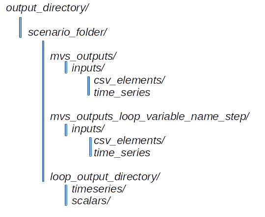
Composition of the output structure within pvcompare.¶

For each scenario, a specific output folder with the name scenario_name is created. All outputs are saved into this scenario_folder. When running apply_mvs() all outputs created by mvs are saved into the folder mvs_outputs. When running loop_mvs() a loop output directory with the additional information of the variable name that is looped over, is created. Within this loop_output_directory all time series and all scalars are copied into specific folders and named with their specific looping step. Additionally all mvs_outputs are saved into a folder with the name `mvs_outputs_loop_variable_name_step’, so that the specific steps can be analyzed easily in separate. For each scenario multiple loops can be applied.

The following image shows an example output directory with specific names of the folders. In this example the function apply_mvs() was run. Further one loop for specific costs over two values (500, 600) was executed.

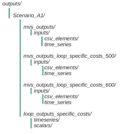
Example output structure of pvcompare with one loop over specific costs.¶

Definition of KPIs¶

KPIs, which were calculated from the outputs of the simulation, are stored in Scalars. The main ones used to interpret the results of simulated scenarios are presented in this section.

Self-consumption also onsite energy fraction is defined as the fraction of all locally generated energy that is consumed by the system itself to the system’s total local generation:

$Self\_Consumption &=\frac{\sum_{i} {E_{generation} (i)} - E_{gridfeedin}(i) - E_{excess}(i)}{\sum_{i} {E_{generation} (i)} } &Self Consumption \epsilon \text{[0,1]}$

The degree of autonomy is used to describe all locally generated energy that is consumed by the system over the system’s total demand:

$Degree\_Of\_Autonomy &=\frac{\sum_{i} {E_{generation} (i)} - E_{gridfeedin}(i) - E_{excess}(i)}{\sum_i {E_{demand} (i)}} &Degree of Autonomy \epsilon \text{[0,1]}$

With the degree of net zero energy , the margin between grid feed-in and grid consumption is compared to the overall demand:

$Degree\_Of\_Net\_Zero\_Energy = 1 + \frac{\sum_{i} E_{gridfeedin}(i) - E_{consumption,provider}(i)}{\sum_{i} E_{demand} (i)}$

Please see the section Outputs of the MVS simulation / Technical data of MVS’s documentation to learn more about the degree of net zero energy.