Model assumptions¶

The energy system optimization implemented in pvcompare is a linear optimization that minimizes the costs of the energy system. Depending on the input parameters single components or all components of the energy system underlie an investment optimization. Certain constraints like a maximum installed capacity, a maximum amount of greenhouse gas / CO₂ emissions or the requirement of forming a net zero energy (NZE) community, if applied, have to be met. Check out the model equations and model assumptions of MVS for detailed information.

Local energy sytem¶

Building assumptions¶

The following paragraph is mostly taken from the work of Haas, Steinbach, Gering & Möller, 2021.

The analyzed local energy system is assumed to belong to an urban neighbourhood with a specific number of buildings. The calculation of the demand profiles are based on standard load profiles that are typically generated for 500-100 hoseholds. The functionalities for calculating the demand profiles of pvcompare, which are introdcued in Electricity and heat demand modeling. These load profiles are flattened, compared to profiles of single households. In order to meet the required number of households, we assume a number of 20 houses by default for our simulations with variable number of storeys and a fixed number of 8 flats per storey. For 5 storey buildings this counts up to 800 households while for 3 storey buildings this counts up to 480 households. The amount of buildings, households per storey, number of people per household and further parameters can be adjusted in the inputs file building_parameters.csv.

The stardard building is constructed with defined building parameters, such as

length south façade
length eastwest façade
total storey area
hight of storey
population per storey

The construction of the building, as well as the available façades for PV usage are based on the research of Hachem, 2014.

The following paragraph is mostly taken from the work of Haas, Steinbach, Gering & Möller, 2021.

The default building parameters are based on the following assumptions that have been adopted from Hachem, 2014: Each storey (with a total area of 1232m²) is divided into 8 flats of 120m² each. The rest of the storey area is used for hallway and staircases etc. Each of the 8 flats is inhabited by 4 people, meaning in average 30m² per person (it is assumed that a NZE building is operated efficiently). Therefore the number of persons per storey is set to 32.

All building parameters can be adjusted in the inputs file building_parameters.csv.

Exploitation for PV Installation¶

The following paragraphs are mostly taken from the work of Haas, Steinbach, Gering & Möller, 2021.

In general we assume an urban environment that allows high solar exposure without shading from surrounding buildings or trees. It is assumed that PV systems can cover “50% of the south façade area, starting from the third floor up, and 80% of the east and west façades.” (Hachem, 2014.) The façades of the first two floors are discarded for PV installation because of shading.

It is possible to simulate a gable roof as well as a flat roof. For the gable roof it is assumed that only the south facing area is used for PV installations. Assuming an elevation of 45°, the gable roof area facing south equals 70% of the total floor area.

For a flat roof, the area available to PV installations is assumed to be 40% of the total floor area, due to shading between the modules (see Energieatlas).

Maximum Capacity¶

The following paragraph is mostly taken from the work of Haas, Steinbach, Gering & Möller, 2021.

With the help of the calculated available area for PV exploitation, the maximum capacity can be evaluated. The maximum capacity, given in the unit of kWp, depends on the size and the peak power of the specific PV technology. It serves as a limit (constraint) for the investment optimization. It is calculated as follows:

$\text{maxCap} = ( \text{available area } / \text{module size } ) \cdot \text{module peak power}$

PV Modeling¶

pvcompare provides the possibility to calculate feed-in time series for the following PV technologies under real world conditions:

flatplate silicon PV module (SI)
hybrid CPV (concentrator-PV) module: CPV cells mounted on a flat plate SI module (CPV)
multi-junction perovskite/silicon module (PeroSi)

While the SI module feed-in time series is completely calculated with pvlib , unique models were developed for the CPV and PeroSi technologies. The next sections will provide a detailed description of the different modeling approaches.

1. SI¶

The silicone module parameters are loaded from cec module database. The module selected by default is the “Aleo_Solar_S59y280” module with a 17% efficiency.

The time series is calculated by making usage of the Modelchain functionality in pvlib. In order to make the results compareable for real world conditions the following methods are selected from modelchain object :

aoi_model=”ashrae”
spectral_model=”first_solar”
temperature_model=”sapm”
losses_model=”pvwatts”

2. CPV¶

Parts of this section are taken from the work of Haas, Steinbach, Gering & Möller, 2021.

The CPV technology that is used in the pvcompare simulations is a hybrid micro-Concentrator module with integrated planar tracking and diffuse light collection of the company INSOLIGHT. The following image describes the composition of the module.

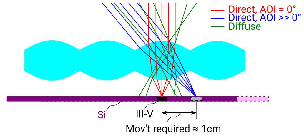
composition scheme of the hybrid module. Direct beam irradiance is collected by 1mm III-V cells, while diffuse light is collected by the Si cell. For AOI not equal to 0°, the biconvex lens maintains a tight but translating focus. A simple mechanism causes the backplane to follow the focal point (see Askins et al., 2019).¶

“The Insolight technology employs a biconvex lens designed such that focusing is possible when the angle of incidence (AOI) approaches 60°, although the focal spot does travel as the sun moves and the entire back plane is translated to follow it, and maintain alignment. The back plane consists of an array of commercial triple junction microcells with approximately 42% efficiency combined with conventional 6” monocrystalline Silicon solar cells. The microcell size is 1mm and the approximate geometric concentration ratio is 180X. Because the optical elements are refractive, diffuse light which is not focused onto the III-V cells is instead collected by the Si cells, which cover the area not taken up by III-V cells. Voltages are not matched between III- V and Si cells, so a four terminal output is provided.” (Askins et al., 2019)

Modeling the hybrid CPV system¶

The model of the cpv technology is outsourced from pvcompare and can be found in the cpvlib repository. pvcompare contains the wrapper function create_cpv_time_series().

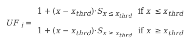
In order to model the dependencies of AOI, temperature and spectrum of the cpv module, the model follows an approach of [Gerstmeier, 2011] previously implemented for CPV in PVSYST. The approach uses the single diode model and adds so called “utilization factors” to the output power to account losses due to spectral and lens temperature variations.

The utilization factors are defined as follows:

$UF = \sum_{i=1}^{n} UF_i \cdot w_i$

“..”¶

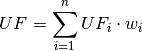
The overall model for the hybrid system is illustrated in the next figure.

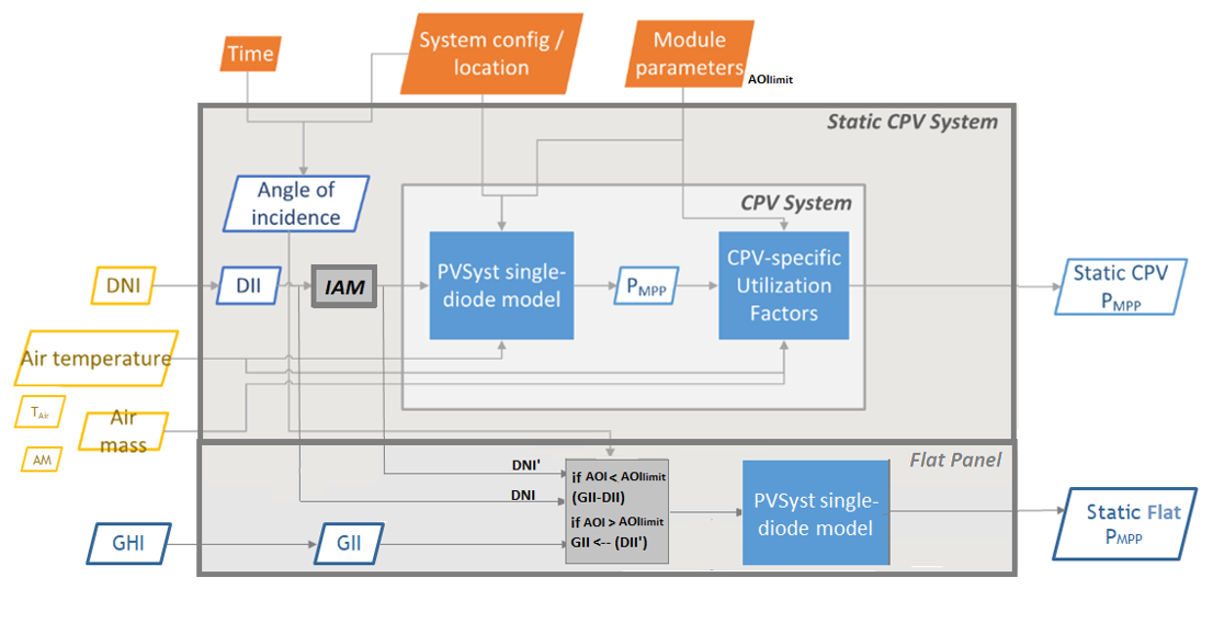
_images/StaticHybridSystem_block_diagram.png

Modeling scheme of the hybrid micro-concentrator module (see cpvlib on github).¶

CPV submodule¶

Input parameters are weather data with AM (air mass), temperature, DNI (direct normal irradiance), GHI (global horizontal irradiance) over time. The CPV part only takes DNI into account. The angle of incidence (AOI) is calculated by pvlib.irradiance.aoi(). Further the pvlib.pvsystem.singlediode() function is solved for the given module parameters. The utilization factors have been defined before by correlation analysis of outdoor measurements. The given utilization factors for temperature and air mass are then multiplied with the output power of the single diode functions. They function as temperature and air mass corrections due to spectral and temperature losses.

Flat plate submodule¶

For AOI < 60° only the diffuse irradiance reaches the flat plate module: GII (global inclined irradiance) - DII (direct inclined irradiance). For Aoi > 60 ° also DII and DHI fall onto the flat plate module. The single diode equation is then solved for all time steps with the specific input irradiance. No module connection is assumed, so CPV and flat plate output power are added up as in a four terminal cell.

Measurement Data¶

The Utilization factors were derived from outdoor measurement data of a three week measurement in Madrid in May 2019. The Data can be found in Zenodo , whereas the performance testing of the test module is described in Askins, et al. (2019).

3. PeroSi¶

Parts of this section are taken from the work of Haas, Steinbach, Gering & Möller, 2021.

The perovskite-silicon cell is a high-efficiency cell that is still in its test phase. Because perovskite is a material that is easily accessible many researchers around the world are investigating the potential of single junction perovskite and perovskite tandem cells cells, which we will focus on here. Because of the early stage of the development of the technology, no outdoor measurement data is available to draw correlations for temperature dependencies or spectral dependencies which are of great impact for multi-junction cells.

Modeling PeroSi¶

The following model for generating an output timeseries under real world conditions is therefore based on cells that were up to now only tested in the laboratory. Spectral correlations were explicitly calculated by applying SMARTS (a Simple Model of the Atmospheric Radiative Transfer of Sunshine) to the given EQE curves of our model. Temperature dependencies are covered by a temperature coefficient for each sub cell. The dependence of AOI is taken into account by SMARTS. The functions for the following calculations can be found in the 3. PeroSi section.

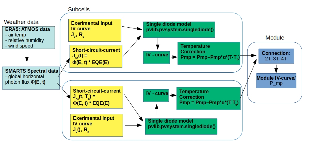
Modeling scheme of the perovskite silicone tandem cell.¶

Input data¶

The following input data is needed:

Weather data with DNI, DHI, GHI, temperature, wind speed
Cell parameters for each sub cell:
- Series resistance (R_s)
- Shunt resistance (R_shunt)
- Saturation current (j_0)
- Temperature coefficient for the short circuit current (α)
- Energy band gap
- Cell size
- External quantum efficiency curve (EQE-curve)

The cell parameters provided in pvcompare are for the cells ([Korte2020]) ith 17 % efficiency and ([Chen2020]) bin 28.2% efficiency. For Chen the parameters R_s, R_shunt and j_0 are evaluated by fitting the IV curve.

Modeling procedure¶

1. weather data The POA_global (plane of array) irradiance is calculated with the pvlib.irradiance.get_total_irradiance() function

2. SMARTS The SMARTS spectrum is calculated for each time step.

2.1. the output values (ghi_for_tilted_surface and photon_flux_for_tilted_surface) are scaled with the ghi from ERA5 weather data. The parameter photon_flux_for_tilted_surface scales linear to the POA_global.

2.2 the short circuit current (J_sc) is calculated for each time step:

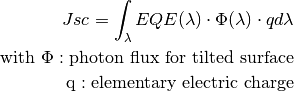
$Jsc = \int_\lambda EQE(\lambda) \cdot \Phi (\lambda) \cdot q d\lambda \text{with } \Phi : \text{photon flux for tilted surface} \text q : \text{elementary electric charge}$

3. The pvlib.pvsystem.singlediode() function is used to evaluate the output power of each sub cell.

3.1 The output power Pmp is multiplied by the number of cells in series

3.2 Losses due to cell connection (5%) and cell to module connection (5%) are taken into account.

The temperature dependency is accounted for by: (see Jost et al., 2020)

$Pmp = Pmp - Pmp \cdot \alpha \cdot (T-T_0)$

In order to get the module output the cell outputs are added up.

3. Normalization¶

For the energy system optimization normalized time series are needed, which can then be scaled to the optimal installation size (in kWp) of the system.

For normalizing the time series calculated for one PV module, the timeseries is devided by the p_mp (power at maximum powerpoint) at standard test conditions (STC). The p_mp of each module can usually be found in the module module sheet.

The normalized timeseries values usually range between 0-1 but can also exceed 1 in case the conditions allow a higher output than the p_mp at STC. The unit of the normalized timeseries is kW/kWp.

Electricity and heat demand modeling¶

Most of this section “Electricity and heat demand modeling” is taken from the work of Haas, Steinbach, Gering & Möller, 2021.

The load profiles of the demand (electricity and heat) are calculated for a given population (calculated from number of storeys), a certain country and year. The profile is generated with the help of oemof.demandlib.

Electricity demand¶

*The following paragraphs are mostly taken from the work of * Haas, Steinbach, Gering & Möller, 2021.

For the electricity demand, the BDEW load profile for households (H0) is scaled with the annual demand of a certain population. It is assumed that the demand of the population is equal to the national residential consumption scaled to the size of this population. Further it is assumed that the electricity demand covers not only all electrical demand for lightning and home appliances but also the energy demand for cooling and cooking. For the latter it is assumed that only electrical energy is used for cooking. Therefore, the share of electrical energy consumption for cooking is subtracted from the total electrical energy consumption before adding the total energy consumption for cooking. Electricity demand does not cover space heating nor hot water. For this reason, the electrical share of space heating and hot water is subtracted from the electricity demand.

The annual electricity profile is calculated by the following procedure:

The national residential electricity consumption for a country is calculated with the following procedure. The data for the total electricity consumption [1] as well as the fractions for space heating (SH) [2], water heating (WH) [3] and cooking [4] [5] are taken from Odyssee Project of Enerdata.

$\text{nec} &= \text{tec}(country, year) \\ &- \text{esh}(country, year) \\ &- \text{ewh}(country, year) \\ &+ \text{tc}(country, year) \\ &- \text{ec}(country, year) \\ \text{with } nec &= \text{national energy consumption} \\ \text{tec} &= \text{total electricity consumption [1]}\\ \text{esh} &= \text{electricity space heating [2]}\\ \text{ewh} &= \text{electricity water heating [3]}\\ \text{tc} &= \text{total cooking [4]}\\ \text{ec} &= \text{electicity cooking [5]}\\$

The population of the country is taken from EUROSTAT.
To obtain the neighbourhood’s total annual demand, the total annual residential electricity demand (step 1) is divided by the country’s population (step 2) and multiplied by the neighbourhood’s population. The population derives from the number of houses, number of storeys and number of people per storage (for building assumptions see Building assumptions).
The load profile is calculated with oemof.demandlib taking holidays into account and then is scaled with the total annual demand of the neighbourhood (step 3).
For multiple countries, the load profile is adapted by hour shifting following the approach of HOTMAPS. For further information see p.127 in HOTMAPS.

Figure Electricity demand shows an exemplary electricty demand for Spain, 2013.

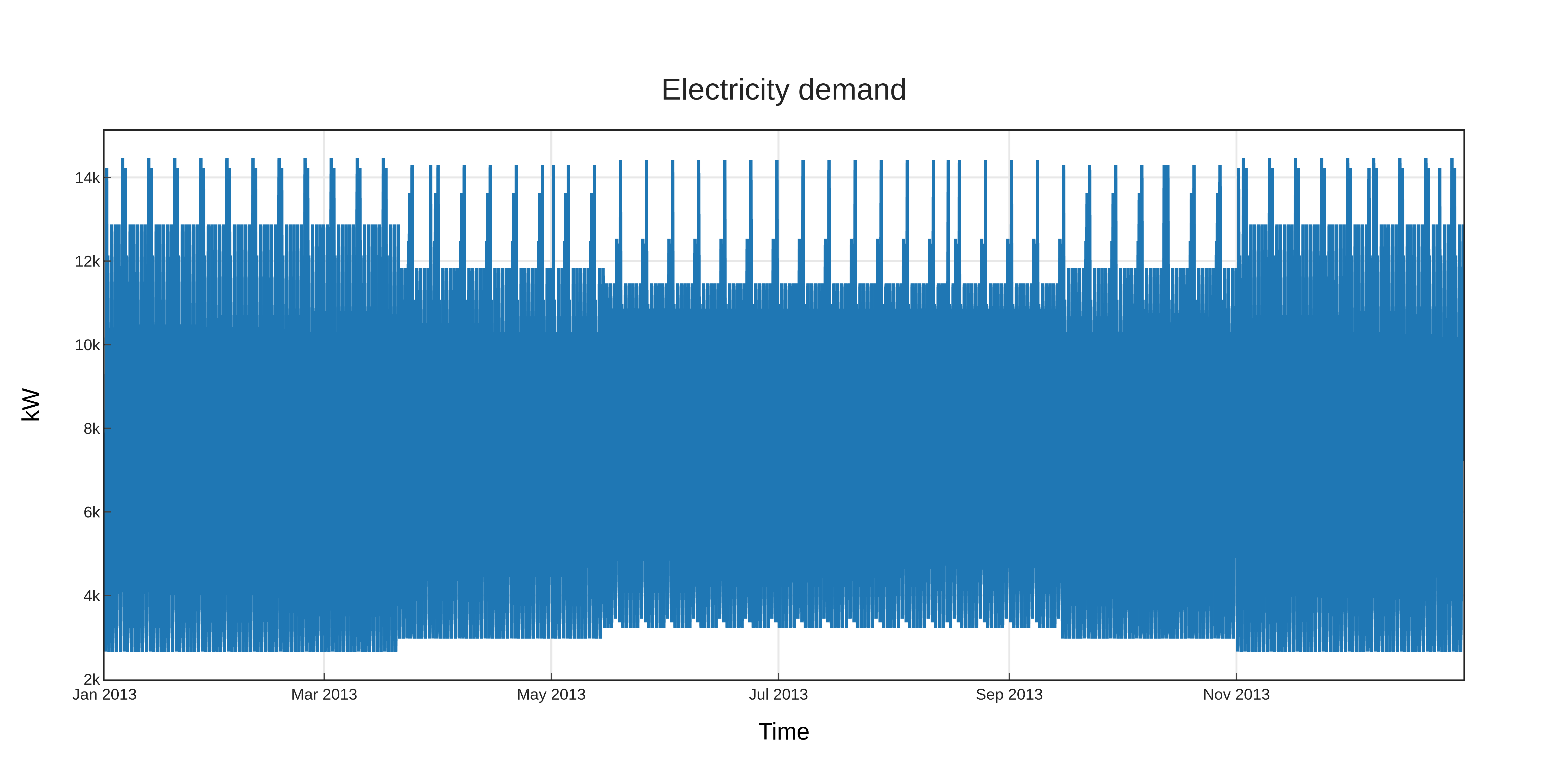
Energy yield per kWp (left) and per m² (right) for Berlin and Madrid in 2014.

Exemplary electricty demand for Spain, 2013.¶

Heat demand¶

The following paragraphs are mostly taken from the work of Haas, Steinbach, Gering & Möller, 2021.

The heat demand of either space heating or space heating and warm water is calculated for a given number of houses with a given number of storeys, a certain country and year. By default only space heating is taken into account. In order to take heat demand from warm water into account the parameter include warm water in pvcompare’s input file building_parameters.csv is set to True. In this case, one heat demand profile is determined which includes the demand for warm water and space heating.

Warning

It is currently not possible to model these two demands separately with two heat demand profiles and, for example, to use different technologies to cover the respective demand. Contributions are very welcome to implement this feature in the future.

To generate the heat demand profiles the BDEW standard load profile is used. This standard load profile is derived for german households. Because there is no other standard load profile available for other countries, the german standard load profile is used for all countries as an approximation. For multiple countries the profile is adapted however by hour shifting.

Due to the characteristics of the sigmoid function used for the calculation of the heat demand profiles, the heat demand never equals zero. Since this does not correspond to the realistic behavior of heat supplied by means of space heating in summer, a heating limit temperature is introduced, above which no heating takes place. The heating limit temperature can be set in building_parameters.csv and is 15 °C by default. In case of space heating, heat demand during summer is removed if the daily mean temperature exceeds the heating limit temperature. The excess heat demand is then distributed equally over the remaining time of the year. In case of a heat demand from space heating and warm water, only the heat demand of the space heating is adjusted as described above.

The standard load profile is scaled with the annual heat demand for the given population, which is derived from the given number of houses and storeys (for assumptions see Building assumptions). The annual heat demand for space heating and warm water is calculated by the following procedure:

The residential heat demand for space heating [6] with or without warm water [7] of a country is taken from the Odyssee Project of Enerdata.
On the lines of the electricity demand, the population of the country is taken from EUROSTAT.
The total residential demand for space heating is divided by the country’s population and multiplied by the neighbourhood’s population. The population derives from the number of houses, number of storeys and number of people per storage (for building assumptions see Building assumptions).
The heat demand profile is calculated with oemof.demandlib for a multi family house and then is scaled with the total annual demand of the neighbourhood (step 3).
Heat demand on days with a daily mean temperature above the heating limit temperature is removed and distributed evenly over the heat demand profile of the remaining time of the year.
For multiple countries, the load profile is adapted by hour shifting following the approach of HOTMAPS. For further information see p.127 in HOTMAPS.

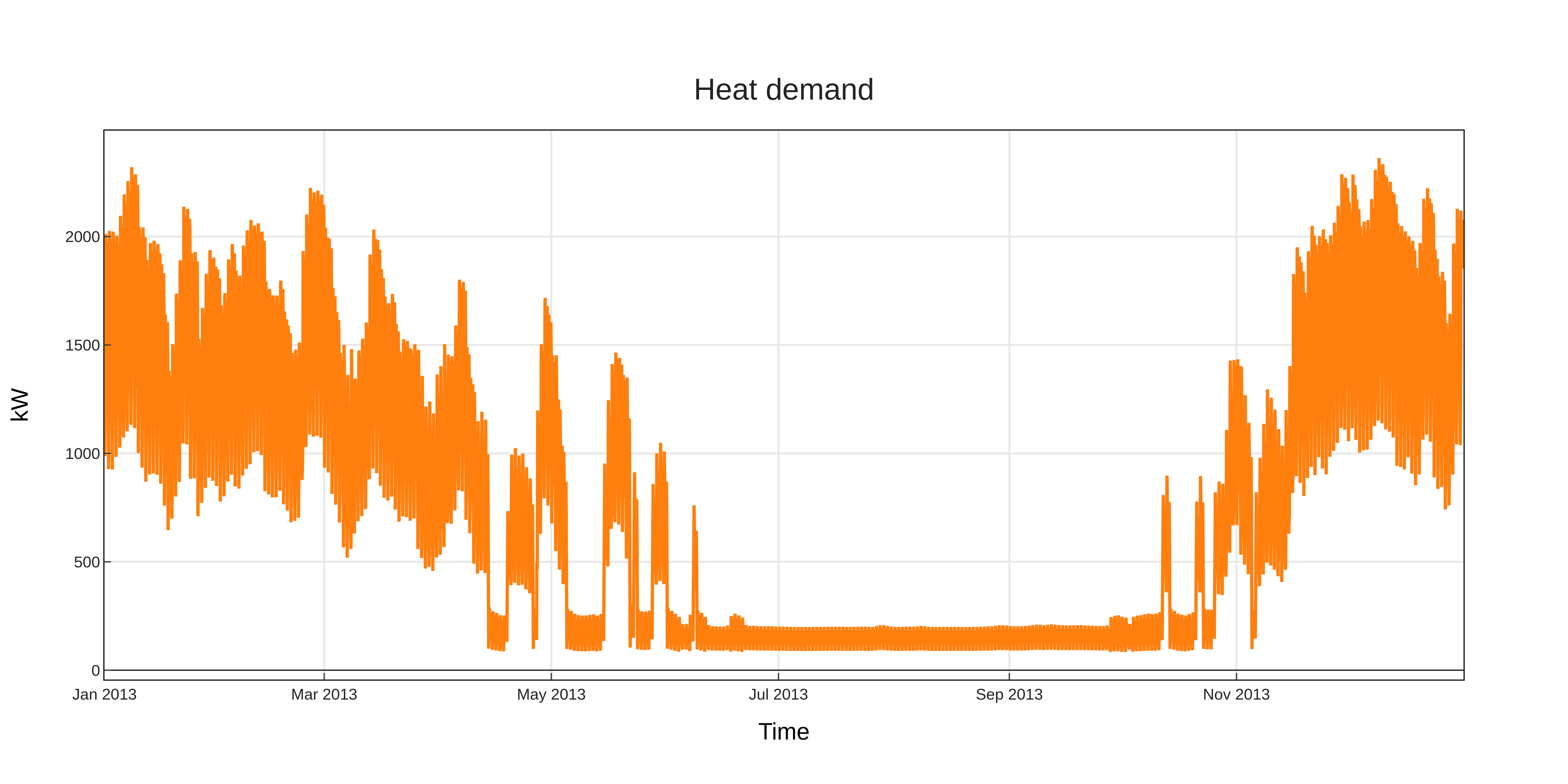
Figure Heat demand sh shows an exemplary heat demand for space heating and figure Heat demand shww the exemplary heat demand from space heating and warm water of Spain, 2013.

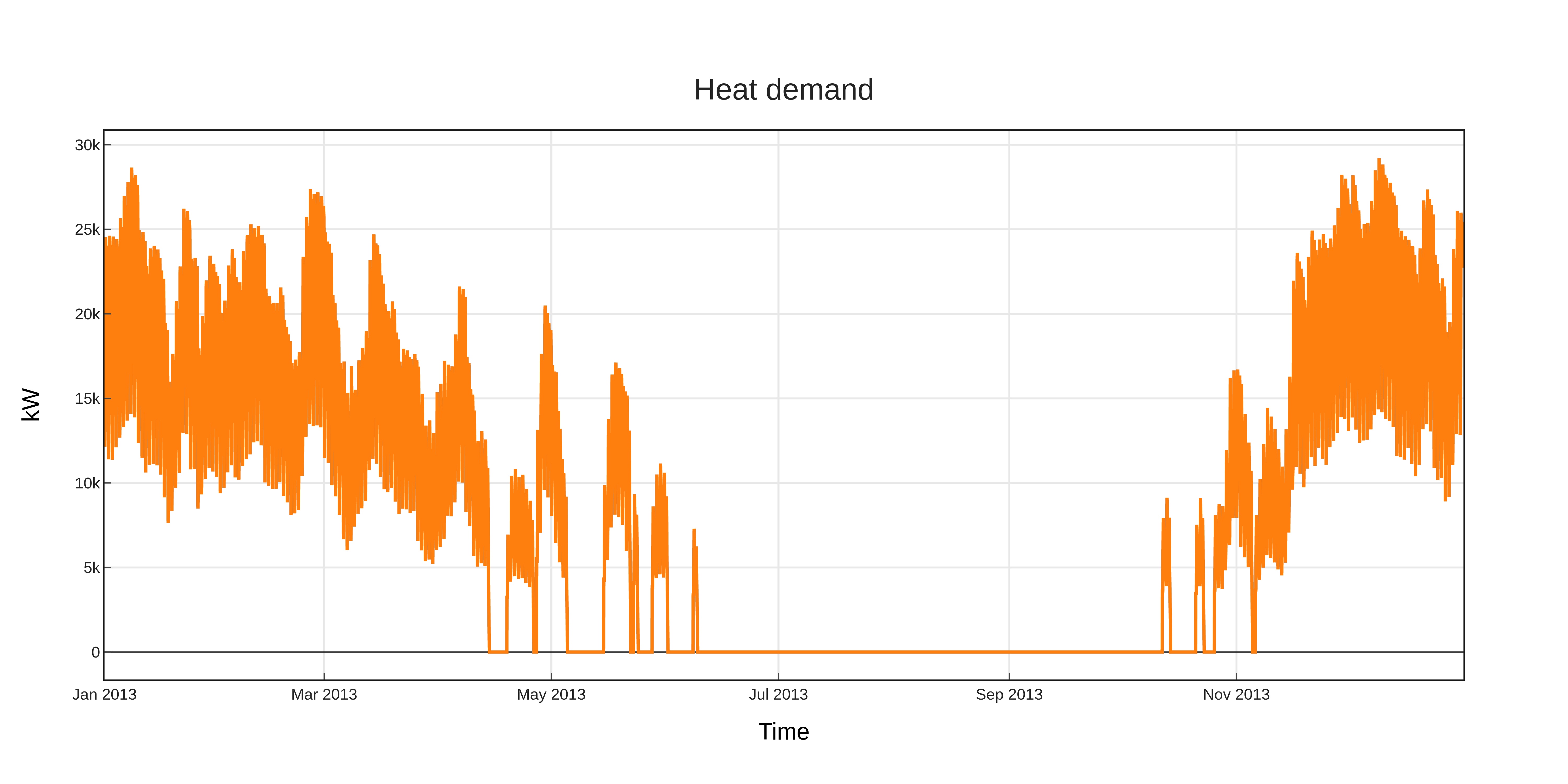
Heat demand in kW for space heating in Madrid in 2013.

Exemplary heat demand for space heating in Madrid, 2013.¶

Heat demand in kW for space heating and warm water in Madrid in 2013.

Exemplary heat demand for space heating and warm water in Madrid, 2013.¶

Heat pump and thermal storage modelling¶

1. Heat pumps and chillers¶

Different types of heat pumps and chillers can be modelled by adjusting their parameters in heat_pumps_and_chillers.csv accordingly.

Parameters which can be adjusted and passed are:

mode: Plant type which can be either heat_pump or chiller

technology: Specific technology of the plant type which can be air-air, air-water or brine-water

quality_grade: Plant-specific scale-down factor to carnot efficiency

temp_high: Outlet temperature / High temperature of heat reservoir

temp_low Inlet temperature / Low temperature of heat reservoir

factor_icing: COP reduction caused by icing (only for heat pumps)

temp_threshold_icing: Temperature below which icing occurs (only for heat pumps)

Please see the documentation on compression heat pumps and chillers of oemof.thermal for further information.

1.1 Heat pumps¶

In case of a heat pump mode and temp_high are required values, while passing temp_low, factor_icing and temp_threshold_icing are optional. Besides either quality_grade or technology has to be passed. The quality grade depends on the technology hence you need to provide a specification of the technology if you want to model the asset from default quality grades. Default values are implemented for the following technologies: air-to-air, air-to-water and brine-to-water. If you provide your own quality grade, passing technology is optional and will be set to an air source technology if passed empty or NaN.

To model an air source heat pump, technology is to be set to either air-air or air-water and the parameter temp_low is passed empty or with NaN. In case you provide your own quality grade, you do not need to specify the technology, since it will be set to the default: air source technology (air-air or air-water). In this case the COP will be calculated from the weather data, to be more exact from the ambient temperature. You can also provide your own time series of temperatures in a separate file as shown in this example of a heat_pumps_and_chillers.csv file:

mode,technology,quality_grade,temp_high,temp_low,factor_icing,temp_threshold_icing
heat_pump,air-water,0.403,"{'file_name': 'temperature_heat_pump.csv', 'header': 'degC', 'unit': ''}",None,None

(In this example temperatures are provided in temperature_heat_pump.csv, with degC as header of the column containing the temperatures.)

To model a water or brine source heat pump, you can either

pass a time series of temperatures with a separate file as shown in the example below or
mode,technology,quality_grade,temp_high,temp_low,factor_icing,temp_threshold_icing heat_pump,water-water,0.45,"{'file_name': 'temperatures_heat_pump.csv', 'header': 'degC', 'unit': ''}",None,None
(In this example temperatures are provided in temperature_heat_pump.csv, with degC as header of the column containing the temperatures.)

pass a numeric with temp_low to model a constant inlet temperature:

mode,technology,quality_grade,temp_high,temp_low,factor_icing,temp_threshold_icing
heat_pump,brine-water,0.53,50,16,None,None
(In this example with constant inlet temperature temp_low)

To model a brine source heat pump from an automatically calculated ground temperature, technology is to be set to brine-water and the parameter temp_low is passed empty or with NaN:

mode,technology,quality_grade,temp_high,temp_low,factor_icing,temp_threshold_icing
heat_pump,brine-water,0.53,50,,None,None
(In this example without passed inlet temperature temp_low)

In this case the COP will be calculated from the mean yearly ambient temperature, as an simplifying assumption of the ground temperature according to brandl_energy_2006

1.2 Chillers¶

Warning

At this point it is not possible to run simulations with a chiller. Adjustments need to be made in add_sector_coupling function of heat_pump_and_chiller.py.

Modelling a chiller is carried out analogously. Here mode and temp_low are required values, while passing temp_high is optional. The parameters factor_icing and temp_threshold_icing have to be passed empty or as NaN or None.

The quality grade depends on the technology hence you need to provide a specification of the technology if you want to model the asset from default quality grade. So far there is only one default value implemented for an air-to-air chiller’s quality grade. It has been obtained from monitored data of the GRECO project. If you provide your own quality grade, passing technology is optional and will be set to an air source technology if passed empty or NaN.

To model an air source chiller, technology is to be set to air-air and the parameter temp_high is passed empty or with NaN. In case you provide your own quality grade, you do not need to specify the technology, since it will be set to the default: air source technology (air-air). In this case the EER will be calculated from the weather data, to be more exact from the ambient temperature. You can also provide your own time series of temperatures in a separate file as in this example of a heat_pumps_and_chillers.csv file:

mode,technology,quality_grade,temp_high,temp_low,factor_icing,temp_threshold_icing
chiller,air-air,0.3,"{'file_name': 'temperatures_chiller.csv', 'header': 'degC', 'unit': ''}",15,None,None

(In this example temperatures are provided in temperature_chiller.csv, with degC as header of the column containing the temperatures.)

To model a water or brine source chiller, you can either

provide a time series of temperatures in a separate file as shown in the example below or
mode,technology,quality_grade,temp_high,temp_low,factor_icing,temp_threshold_icing chiller,water-water,0.45,"{'file_name': 'temperatures_chiller.csv', 'header': 'degC', 'unit': ''}",15,None,None
(In this example temperatures are provided in temperature_chiller.csv, with degC as header of the column containing the temperatures.)
pass a numeric with temp_high to model a constant outlet temperature:
mode,technology,quality_grade,temp_high,temp_low,factor_icing,temp_threshold_icing chiller,water-water,0.3,25,15,None,None
(In this example with constant outlet temperature temp_high)

2. Stratified thermal storage¶

In order to model a stratified thermal energy storage pvcompare provides precalculations of this component. The storage’s parameters in storage_02.csv

installedCap,

efficiency,

fixed_losses_relative and

fixed_losses_absolute

can be obtained, if not provided by the user, orientating on the stratified thermal storage component of oemof.thermal.

The precalculations are done passing the following input parameters with the file stratified_thermal_storage.csv, which is located in the pvcompare’s iputs directory:

height

diameter

temp_h

temp_c

s_iso

lamb_iso

alpha_inside

alpha_outside

Please see stratified_thermal_storage.csv and the documentation of oemof.thermal for further explanations of these parameters. The assumptions made setting these parameters in pvcompare, based on a manufacturer’s prototype of a stratified thermal storage, are summed up in stratified_thermal_storage.csv.

For further information on how the stratified thermal storage is modeled in the MVS, please see the documentation of the MVS.

2.1 Installed Capacity¶

The calculations are implemented within Stratified thermal storage. For an investment optimization the height of the storage should be left open and installedCap should be set to 0 or NaN. If you do a simulation with a fixed storage capacity, you can either

set a numeric for installedCap:
,unit,storage capacity,input power,output power installedCap,kWh,100,0,0
(In this example the installed capacity is provided as a numeric within storage_02.csv)
or use the precalculations with leaving installedCap open or set to NaN and passing a numeric with the height parameter:
,unit,storage capacity,input power,output power installedCap,kWh,,0,0
(In this example the installed capacity is left open within storage_02.csv)
var_name,var_value,var_unit height,2.04,m diameter,0.79,m temp_h,40,degC temp_c,34,degC s_iso,100,mm lamb_iso,0.03,W/(m*K) alpha_inside,4.3,W/(m2*K) alpha_outside,3.17,W/(m2*K)
(In this example the height is provided as a numeric within stratified_thermal_storage.csv)

The parameters U-value, volume and surface of the storage, which are required to calculate installedCap, are precalculated as well within Stratified thermal storage.

2.2 Efficiency¶

The efficiency $\eta$ of the storage is calculated as follows:

$\eta = 1 - loss{\_}rate$

with the parameter loss_rate, which is calculated in Stratified thermal storage using the function calculate_losses of oemof.thermal. Please see the oemof.thermal examples and the documentation for further information.

2.3 Fixed losses relative and absolute¶

Besides the relative thermal loss of storage content within one timestep [-] expressed by the loss_rate, fixed losses as share of nominal storage capacity [-] and fixed absolute losses independent of storage content or nominal storage capacity [kWh] can be passed as well (cf. oemof.thermal’s documentation on the stratified thermal storage). You can model the stratified thermal storage with fixed thermal losses by either providing

a numeric value:

,unit,storage capacity,input power,output power
fixed_thermal_losses_relative,factor,0.001,NA,NA
fixed_thermal_losses_absolute,kWh,0.00001,NA,NA
(In this example the fixed thermal losses are provided as a numeric within storage_02.csv)

your own time series with numeric values:

,unit,storage capacity,input power,output power
fixed_thermal_losses_relative,factor,"{'file_name': 'my_fixed_losses_relative.csv', 'header': 'no_unit', 'unit': ''}",,
fixed_thermal_losses_absolute,kWh,"{'file_name': 'my_fixed_losses_absolute.csv', 'header': 'kWh', 'unit': ''}",,
(In this example the fixed thermal losses are provided as an own time series using CSV files within storage_02.csv with no_unit as header of the column with the fixed losses relative and kWh as header of the column with the fixed losses absolute)

or using pvcompare’s precalculation as described above:
,unit,storage capacity,input power,output power fixed_thermal_losses_relative,factor,"{'file_name': 'None', 'header': 'no_unit', 'unit': ''}",, fixed_thermal_losses_absolute,kWh,"{'file_name': 'None', 'header': 'kWh', 'unit': ''}",,
(In this example the fixed thermal losses are calculated in Stratified thermal storage and written to the field 'file_name' in storage_02.csv with no_unit as header of the column with the fixed losses relative and kWh as header of the column with the fixed losses absolute)

[1] Enerdata: Electricity consumption of residential sector. https://odyssee.enerdata.net/database/

[2] Enerdata: Electricity consumption of residential for space heating. https://odyssee.enerdata.net/database/

[3] Enerdata: Electricity consumption of households for water heating. https://odyssee.enerdata.net/database/

[4] Enerdata: Final consumption of residential for cooking. https://odyssee.enerdata.net/database/

[5] Enerdata: Electricity consumption of residential for cooking. https://odyssee.enerdata.net/database/

[6] Enerdata: Final consumption of residential for space heating. https://odyssee.enerdata.net/database/

[7] Enerdata: Final consumption of households for water heating. https://odyssee.enerdata.net/database/