Welcome to the documentation of pvcompare!¶

pvcompare is a model for comparing the benefits of different PV technologies in a specified local energy system in different energy supply scenarios.

Deprecated:

pvcompare¶

Introduction¶

pvcompare is a model that compares the benefits of different PV technologies in a specified energy system by running an energy system optimization. This model concentrates on the integration of PV technologies into local energy systems but could easily be enhanced to analyse other conversion technologies.

The functionalities include

calculation of an area potential for PV on roof-tops and facades based on building parameters,
calculation of heat and electricity demand profiles for a specific amount of people living in these buildings,
calculation of PV feed-in time series for a set of PV installations on roof-tops and facades incl. different technologies,
- all technologies in the database of pvlib,
- a specific concentrator-PV module, and
- a module of silicon-perovskite cells,
calculation of temperature dependent COPs or respectively EERs for heat pumps and chillers,
preparation of data and input files for the energy system optimization,
a sensitivity analysis for input parameters and
visualisations for the comparison of different technologies.

The model is being developed within the scope of the H2020 project GRECO. The energy system optimization is based on the oemof-solph python package, which pvcompare calls via the Multi-Vector Simulator (MVS), a tool for assessing and optimizing Local Energy Systems (LES).

Documentation¶

The full documentation can be found at readthedocs.

Installation¶

To install pvcompare follow these steps:

Clone pvcompare and navigate to the directory \pvcompare containing the setup.py and requirements.txt:

git clone git@github.com:greco-project/pvcompare.git
cd pvcompare

Install the package:

pip install -e .

For the optimization you need to install a solver. Your can download the open source cbc-solver from https://ampl.com/dl/open/cbc/ . Please follow the installation steps in the oemof installation instructions. You also find information about other solvers there.

Examples and basic usage¶

The basic usage of pvcompare is explained in the documentation in section Basic usage of pvcompare.

Contributing¶

We are warmly welcoming all who want to contribute to pvcompare. Please read our Contributing Guidelines.

Basic usage of pvcompare¶

Run a simulation¶

You can easily run a simulation with pvcompare by running the file TODO (adjust after decision in #164). More information to follow.

Define your own components and parameters¶

pvcompare provides you with templates and default parameters for your simulations. However, you can also define your own energy system, choose different parameters and/or change the settings.

Please refer to Simulating with the MVS to learn how to work with the input csv files and how to provide your own time series. In pvcompare these files are by default stored in the directory data/mvs_inputs. You can define another input directory by providing the parameter mvs_input_directory to the main() and apply_mvs() functions. Please note that pvcompare only works with csv files but not with json files.

Further parameters are stored in the data/inputs directory. You can adapt this directory by providing the parameter input_directory to the main() and apply_mvs() functions. Especially interesting for adapting your simulations will be:

pv_setup.csv: Definition of PV assets (technology, tilt angle, azimuth angle, roof-top or facade installation)
building_parameters.csv: Definition of characteristics of the building type that should be considered in the simulation.
heat_pumps_and_chillers.csv: Definition of characteristics of the heat pumps and chillers in the simulated energy system.

A full description of the parameters can be found in the section Parameters of pvcompare: Definitions and Default Values.

Download ERA5 weather data¶

Info follows, see #68.

Add a sensitivy to your simulations¶

Here follows a description of how to use the automated_loop() functionality.

Model assumptions¶

Building assumptions¶

The demand profiles that are introduced in the next sections are based on so called standard load profiles. These standard load profiles are generated for around 500-1000 Household, therefore the curve is flattened and cannot be compares to the load curve of a single household. This is why the pvcompare simulations are based on NZE communities reather than a single NZE building. As a consequence all simulations are run over a number of 400 identical buildings. In order to interpret the simulation results for a single building, the total demand / production can be devided by 400. (TODO: is this correct??)

In general we assume an urban environment that allows high solar exposure without shading from surrounding buildings or trees.

The stardard building is constructed with defined building parameters, such as

length south facade
length eastwest facade
total storey area
hight of storey
population per storey

All building parameters are contained in ‘data/static_inputs/building_parameters.csv’. The construction of the buidling, as well as the available facades for PV usage are based on the research of Hachem, 2014.

The default building parameters are based on the following assumptions that have been adopted from Hachem, 2014:

Each storey (with a total area of 1232 m²) is defided into 8 flats, each 120 m². The rest of the storey area is used for hallway and staircases etc. Each of the 8 flats is inhabited by 4 people, meaning in average 30m² per person (it is assumed that a NZE building is operated efficiently). Therefore the number of persons per storey is set to 32.

Exploitation for PV Installation¶

It is assumed that PV systems can cover “50% of the south façade area, starting from the third floor up, and 80% of the east and west façades.” (Hachem, 2014.) The facades of the first two floors are discarded for PV installation because of shading.

It is possible to simulate a gable roof as well as a flat roof. For the gable roof it is assumed that only the south facing area is used for PV installations. Assuming an elevation of 45°, the gable roof area facing south equals 70% of the total floor area.

For a flat roof area available to PV installations is assumed to be 40% of the total floor area, due to shading between the modules (see Energieatlas.

Maximum Capacity¶

With the help of the calculated available area for PV exploitation, the maximum capacity can be calculated. The maximum capacity, given in the unit of kWp, depends on the size and the efficiency of the specific PV technology. It serves as a limit for the investment optimization with MVS. It is calculated as follows:

$\text{maxCap} = ( \text{available area } / \text{module size } ) \cdot \text{module peak power}$

PV Modeling¶

pvcompare provides the possibility to calculate feed-in time series for the following PV technologies under real world conditions:

flatplate silicon PV module (SI)
hybrid CPV (concentrator-PV) module: CPV cells mounted on a flat plate SI module (CPV)
multi-junction perovskite/silicon module (PeroSi)

While the SI module feed-in time series is completely calculated with pvlib , unique models were developed for the CPV and PeroSi technologies. The next sections will provide a detailed description of the different modeling approaches.

1. SI¶

The silicone module parameters are loaded from cec module database. The module selected by default is the “Aleo_Solar_S59y280” module with a 17% efficiency. But any other module can be selected.

The time series is calculated by making usage of the Modelchain functionality in pvlib. In order to make the results compareable for real world conditions the following methods are selected from modelchain object :

aoi_model=”ashrae”
spectral_model=”first_solar”
temperature_model=”sapm”
losses_model=”pvwatts”

2. CPV¶

The CPV technology that is used in the pvcompare simulations is a hybrid micro-Concentrator module with integrated planar tracking and diffuse light collection of the company INSOLIGHT. The following image describes the composition of the module.

composition scheme of the hybrid module. Direct beam irradiance is collected by 1mm III-V cells, while diffuse light is collected by the Si cell. For AOI not equal to 0°, the biconvex lens maintains a tight but translating focus. A simple mechanism causes the backplane to follow the focal point (see Askins et al., 2019).

“The Insolight technology employs a biconvex lens designed such that focusing is possible when the angle of incidence (AOI) approaches 60°, although the focal spot does travel as the sun moves and the entire back plane is translated to follow it, and maintain alignment. The back plane consists of an array of commercial triple junction microcells with approximately 42% efficiency combined with conventional 6” monocrystalline Silicon solar cells. The microcell size is 1mm and the approximate geometric concentration ratio is 180X. Because the optical elements are refractive, diffuse light which is not focused onto the III-V cells is instead collected by the Si cells, which cover the area not taken up by III-V cells. Voltages are not matched between III- V and Si cells, so a four terminal output is provided.” (Askins et al., 2019)

Modeling the hybrid CPV system¶

The model of the cpv technology is outsourced from pvcompare and can be found in the cpvlib repository. pvcompare contains the wrapper function create_cpv_time_series().

In order to model the dependencies of AOI, temperature and spectrum of the cpv module, the model follows an approach of [Gerstmeier, 2011] previously implemented for CPV in PVSYST. The approach uses the single diode model and adds so called “utilization factors” to the output power to account losses due to spectral and lens temperature variations.

The utilization factors are defined as follows:

$UF = \sum_{i=1}^{n} UF_i \cdot w_i$

“..”

The overall model for the hybrid system is illustrated in the next figure.

_images/StaticHybridSystem_block_diagram.png

Modeling scheme of the hybrid micro-concentrator module (see cpvlib on github).

CPV submodule¶

Input parameters are weather data with AM (air mass), temperature, DNI (direct normal irradiance), GHI (global horizontal irradiance) over time. The CPV part only takes DNI into account. The angle of incidence (AOI) is calculated by pvlib.irradiance.aoi(). Further the pvlib.pvsystem.singlediode() function is solved for the given module parameters. The utilization factors have been defined before by correlation analysis of outdoor measurements. The given utilization factors for temperature and air mass are then multiplied with the output power of the single diode functions. They function as temperature and air mass corrections due to spectral and temperature losses.

Flat plate submodule¶

For AOI < 60° only the diffuse irradiance reaches the flat plate module: GII (global inclined irradiance) - DII (direct inclined irradiance). For Aoi > 60 ° also DII and DHI fall onto the flat plate module. The single diode equation is then solved for all time steps with the specific input irradiance. No module connection is assumed, so CPV and flat plate output power are added up as in a four terminal cell.

Measurement Data¶

The Utilization factors were derived from outdoor measurement data of a three week measurement in Madrid in May 2019. The Data can be found in Zenodo , whereas the performance testing of the test module is described in Askins, et al. (2019).

2. PeroSi¶

The perovskite-silicon cell is a high-efficiency cell that is still in its test phase. Because perovskite is a material that is easily accessible many researchers around the world are investigating the potential of single junction perovskite and perovskite tandem cells cells, which we will focus on here. Because of the early stage of the development of the technology, no outdoor measurement data is available to draw correlations for temperature dependencies or spectral dependencies which are of great impact for multi-junction cells.

Modeling PeroSi¶

The following model for generating an output timeseries under real world conditions is therefore based on cells that were up to now only tested in the laboratory. Spectral correlations were explicitly calculated by applying SMARTS (a Simple Model of the Atmospheric Radiative Transfer of Sunshine) to the given EQE curves of our model. Temperature dependencies are covered by a temperature coefficient for each sub cell. The dependence of AOI is taken into account by SMARTS. The functions for the following calculations can be found in the PSI time series section.

Modeling scheme of the perovskite silicone tandem cell.

Input data¶

The following input data is needed:

Weather data with DNI, DHI, GHI, temperature, wind speed
Cell parameters for each sub cell:
- Series resistance (R_s)
- Shunt resistance (R_shunt)
- Saturation current (j_0)
- Temperature coefficient for the short circuit current (α)
- Energy band gap
- Cell size
- External quantum efficiency curve (EQE-curve)

The cell parameters provided in pvcompare are for the cells ([Korte2020]) ith 17 % efficiency and ([Chen2020]) bin 28.2% efficiency. For Chen the parameters R_s, R_shunt and j_0 are evaluated by fitting the IV curve.

Modeling procedure¶

1. weather data The POA_global (plane of array) irradiance is calculated with the pvlib.irradiance.get_total_irradiance() function

2. SMARTS The SMARTS spectrum is calculated for each time step.

2.1. the output values (ghi_for_tilted_surface and photon_flux_for_tilted_surface) are scaled with the ghi from ERA5 weather data. The parameter photon_flux_for_tilted_surface scales linear to the POA_global.

2.2 the short circuit current (J_sc) is calculated for each time step:

$Jsc = \int_\lambda EQE(\lambda) \cdot \Phi (\lambda) \cdot q d\lambda \text{with } \Phi : \text{photon flux for tilted surface} \text q : \text{elementary electric charge}$

3. The pvlib.pvsystem.singlediode() function is used to evaluate the output power of each sub cell.

3.1 The output power Pmp is multiplied by the number of cells in series

3.2 Losses due to cell connection (5%) and cell to module connection (5%) are taken into account.

The temperature dependency is accounted for by: (see Jost et al., 2020)

$Pmp = Pmp - Pmp \cdot \alpha \cdot (T-T_0)$

In order to get the module output the cell outputs are added up.

3. Normalization¶

For the energy system optimization normalized time series are needed, which can then be scaled to the optimal installation size (in kWp) of the system.

For normalizing the time series calculated for one PV module, the timeseries is devided by the p_mp (power at maximum powerpoint) at standard test conditions (STC). The p_mp of each module can usually be found in the module module sheet.

The normalized timeseries values usually range between 0-1 but can also exceed 1 in case the conditions allow a higher output than the p_mp at STC. The unit of the normalized timeseries is kW/kWp.

Electricity and heat demand modeling¶

The load profiles of the demand (electricity and heat) are calculated for a given population (calculated from number of storeys), a certain country and year. The profile is generated with the help of oemof.demandlib.

Electricity demand¶

For the electricity demand, the BDEW load profile for households (H0) is scaled with the annual demand of a certain population. Therefore the annual electricity demand is calculated by the following procedure:

the national residential electricity consumption for a country is calculated with the following procedure. The data for the total electricity consumption as well as the fractions for space heating (SH), water heating (WH) and cooking are taken from EU Building Database.

$\text{nec} &= \text{tec}(country, year) \\ &- \text{esh}(country, year) \\ &- \text{ewh}(country, year) \\ &+ \text{tc}(country, year) \\ &- \text{ec}(country, year) \\ \text{with } nec &= \text{national energy consumption} \\ \text{tec} &= \text{total electricity consumption} \\ \text{esh} &= \text{electricity space heating} \\ \text{ewh} &= \text{electricity water heating} \\ \text{tc} &= \text{total cookin}g \\ \text{ec} &= \text{electicity cooking} \\$

the population of the country is requested from EUROSTAT.
the total residential demand is divided by the countries population and multiplied by the house population. The house population is calculated by the number of storeys and the number of people per storey.
The load profile is shifted due to country specific behaviour following the approach of HOTMAPS. For further information see p.127 in HOTMAPS.

Figure Electricity demand shows an exemplary electricty demand for Spain, 2013.

Energy yield per kWp (left) and per m² (right) for Berlin and Madrid in 2014.

Exemplary electricty demand for Spain, 2013.

Heat demand¶

The heat demand is calculated for a given number of houses with a given number of storeys, a certain country and year. The BDEW standard load profile is used. This standard load profile is derived for german households. Because there is no other standard load profiles available for other countries, the german standard load profiles is used for all countries as an approximation.

The standard load profile is scaled with the annual heat demand for the given population. The annual heat demand is calculated by the following procedure:

the residential heat demand for a country is requested from EU Building Database. Only the Space Heating is used in the simulations (TODO: How to include WH).
on the lines of the electricity demand, the population of the country is requested from EUROSTAT.
the total residential demand is divided by the countries population and multiplied by the house population that is calculated by the storeys of the house and the number of people in one storey
The load profile is shifted due to countries specific behaviour following the approach of HOTMAPS. For further information see p.127 in HOTMAPS.

Figure Heat demand shows an exemplary electricty demand for Spain, 2013.

Exemplary heat demand for Spain, 2013.

Heat pump and thermal storage modelling¶

1. Heat pumps and chillers¶

Different types of heat pumps and chillers can be modelled by adjusting their parameters in heat_pumps_and_chillers.csv accordingly.

Parameters which can be adjusted and passed are:

mode: Plant type which can be either heat_pump or chiller

technology: Specific technology of the plant type which can be air-air, air-water or brine-water

quality_grade: Plant-specific scale-down factor to carnot efficiency

temp_high: Outlet temperature / High temperature of heat reservoir

temp_low Inlet temperature / Low temperature of heat reservoir

factor_icing: COP reduction caused by icing (only for heat pumps)

temp_threshold_icing: Temperature below which icing occurs (only for heat pumps)

Please see the documentation on compression heat pumps and chillers of oemof.thermal for further information.

1.1 Heat pumps¶

In case of a heat pump mode and temp_high are required values, while passing temp_low, factor_icing and temp_threshold_icing are optional. Besides either quality_grade or technology has to be passed. The quality grade depends on the technology hence you need to provide a specification of the technology if you want to model the asset from default quality grades. Default values are implemented for the following technologies: air-to-air, air-to-water and brine-to-water. If you provide your own quality grade, passing technology is optional and will be set to an air source technology if passed empty or NaN.

To model an air source heat pump, technology is to be set to either air-air or air-water and the parameter temp_low is passed empty or with NaN. In case you provide your own quality grade, you do not need to specify the technology, since it will be set to the default: air source technology (air-air or air-water). In this case the COP will be calculated from the weather data, to be more exact from the ambient temperature. You can also provide your own time series of temperatures in a separate file as shown in this example of a heat_pumps_and_chillers.csv file:

mode,technology,quality_grade,temp_high,temp_low,factor_icing,temp_threshold_icing
heat_pump,air-water,0.403,"{'file_name': 'temperature_heat_pump.csv', 'header': 'degC', 'unit': ''}",None,None

(In this example temperatures are provided in temperature_heat_pump.csv, with degC as header of the column containing the temperatures.)

To model a water or brine source heat pump, you can either

pass a time series of temperatures with a separate file as shown in the example below or
mode,technology,quality_grade,temp_high,temp_low,factor_icing,temp_threshold_icing heat_pump,water-water,0.45,"{'file_name': 'temperatures_heat_pump.csv', 'header': 'degC', 'unit': ''}",None,None
(In this example temperatures are provided in temperature_heat_pump.csv, with degC as header of the column containing the temperatures.)

pass a numeric with temp_low to model a constant inlet temperature:

mode,technology,quality_grade,temp_high,temp_low,factor_icing,temp_threshold_icing
heat_pump,brine-water,0.53,65,16,None,None
(In this example with constant inlet temperature temp_low)

To model a brine source heat pump from an automatically calculated ground temperature, technology is to be set to brine-water and the parameter temp_low is passed empty or with NaN:

mode,technology,quality_grade,temp_high,temp_low,factor_icing,temp_threshold_icing
heat_pump,brine-water,0.53,65,,None,None
(In this example without passed inlet temperature temp_low)

In this case the COP will be calculated from the mean yearly ambient temperature, as an simplifying assumption of the ground temperature according to brandl_energy_2006

1.2 Chillers¶

Warning

At this point it is not possible to run simulations with a chiller. Adjustments need to be made in add_sector_coupling function of heat_pump_and_chiller.py.

Modelling a chiller is carried out analogously. Here mode and temp_low are required values, while passing temp_high is optional. The parameters factor_icing and temp_threshold_icing have to be passed empty or as NaN or None.

The quality grade depends on the technology hence you need to provide a specification of the technology if you want to model the asset from default quality grade. So far there is only one default value implemented for an air-to-air chiller’s quality grade. It has been obtained from monitored data of the GRECO project. If you provide your own quality grade, passing technology is optional and will be set to an air source technology if passed empty or NaN.

To model an air source chiller, technology is to be set to air-air and the parameter temp_high is passed empty or with NaN. In case you provide your own quality grade, you do not need to specify the technology, since it will be set to the default: air source technology (air-air). In this case the EER will be calculated from the weather data, to be more exact from the ambient temperature. You can also provide your own time series of temperatures in a separate file as in this example of a heat_pumps_and_chillers.csv file:

mode,technology,quality_grade,temp_high,temp_low,factor_icing,temp_threshold_icing
chiller,air-air,0.3,"{'file_name': 'temperatures_chiller.csv', 'header': 'degC', 'unit': ''}",15,None,None

(In this example temperatures are provided in temperature_chiller.csv, with degC as header of the column containing the temperatures.)

To model a water or brine source chiller, you can either

provide a time series of temperatures in a separate file as shown in the example below or
mode,technology,quality_grade,temp_high,temp_low,factor_icing,temp_threshold_icing chiller,water-water,0.45,"{'file_name': 'temperatures_chiller.csv', 'header': 'degC', 'unit': ''}",15,None,None
(In this example temperatures are provided in temperature_chiller.csv, with degC as header of the column containing the temperatures.)
pass a numeric with temp_high to model a constant outlet temperature:
mode,technology,quality_grade,temp_high,temp_low,factor_icing,temp_threshold_icing chiller,water-water,0.3,25,15,None,None
(In this example with constant outlet temperature temp_high)

Parameters of pvcompare: Definitions and Default Values¶

Within the pvcompare/pvcompare/data/ directory, two separate categories of inputs can be observed.

MVS parameters (found in the CSVs within the data/mvs_inputs/csv_elements/ directory)
pvcompare-specific parameters (found in the CSVs within the data/inputs directory)

1. MVS Parameters¶

As pvcompare makes use of the Multi-vector Simulation (MVS) tool, the definitions of all the relevant parameters of MVS can be found in the documentation of MVS.

The values used by default in pvcompare for the above parameters in each CSV, are detailed below. Some parameters can be calculated automatically by pvcompare and do not need to be filled it by hand. These parameters are marked with * auto_calc.

project_data.csv
1. country: str, Spain (the country in which the project is located), * auto_calc
2. label: str, project_data
3. latitude: str, 45.641603 * auto_calc
4. longitude: str, 5.875387 * auto_calc
5. project_id: str, 1
6. project_name: str, net zero energy community
7. scenario_description: str, Simulation of scenario scenario_name
economic_data.csv
1. curency: str, EUR (stands for euro; can be replaced by SEK, if the system is located in Sweden, for instance).
2. discount_factor: factor, 0.06 (most recent data is from 2018, as documented by this market survey.
3. label: str, economic_data
4. project_duration: year, 1 (number of years)
5. tax: factor, 0 (this feature has not been implemented yet, as per MVS documentation)
simulation_settings.csv
1. evaluated_period: days, 365 (number of days), * auto_calc
2. label: str, simulation_settings
3. output_lp_file: bool, False
4. restore_from_oemof_file: bool, False
5. start_date: str, 2013-01-01 00:00:00, * auto_calc
6. store_oemof_results: bool, True
7. timestep: minutes, 60 (hourly time-steps, 60 minutes)
8. display_nx_graph: bool, False
9. store_nx_graph: bool ,True

fixcost.csv

	Unit	distribution_grid	engineering	operation
age_installed	year	10	0	0
development_costs	currency	10	0	0
specific_cost	currency	10	0	4600
label	str	distribution grid infrastructure	R&D, engineering	Fix project operation
lifetime	year	30	20	20
specific_cost_om	currency/year	10	0	0
dispatch_price	currency/kWh	0	0	0

energyConsumption.csv
1. dsm: str, False (dsm stands for Demand Side Management. This feature has not been implement in MVS as of now.)
2. file_name: str, electricity_load.csv
3. label: str, Households
4. type_asset: str, demand
5. type_oemof: str, sink
6. energyVector: str, Electricity
7. inflow_direction: str, Electricity
8. unit: str, kW
energyConversion.csv
1. age_installed: year, 0 (for all components such as charge controllers, inverters, heat pumps, gas boilers)
2. development_costs: currency, 0 (for all components)
3. specific_costs: currency/kW
  
  storage_charge_controller_in and storage_charge_controller_out: 46 (According to this source, a 12 Volts, 80 Amperes Solar Charge Controller costs about 50 USD, which is about 46 €/kW.)
  
  solar_inverter_01: 230 (Per this, the cost of inverters are around 230 Euro/kW.)
  
  heat_pump_air_air_2015: 450 (According to Danish energy agency’s technology data of an air-to-air heat pump [dea_hp_aa] on page 87.)
  
  heat_pump_air_air_2020: 425 (According to dea_hp_aa)
  
  heat_pump_air_air_2030: 316.67 (According to dea_hp_aa)
  
  heat_pump_air_air_2050: 300 (According to dea_hp_aa)
  
  heat_pump_air_water_2015: 1000 (According to Danish energy agency’s technology data of an air-to-air heat pump [dea_hp_aw] on page 89.)
  
  heat_pump_air_water_2020: 940 (According to dea_hp_aw)
  
  heat_pump_air_water_2030: 850 (According to dea_hp_aw)
  
  heat_pump_air_water_2050: 760 (According to dea_hp_aw)
  
  heat_pump_brine_water_2015: 1600 (According to Danish energy agency’s technology data of an air-to-air heat pump [dea_hp_bw] on page 93.)
  
  heat_pump_brine_water_2020: 1500 (According to dea_hp_bw)
  
  heat_pump_brine_water_2030: 1400 (According to dea_hp_bw)
  
  heat_pump_brine_water_2050: 1200 (According to dea_hp_bw)
  
  natural_gas_boiler_2015: 320 (According to Danish energy agency’s technology data of a natural gas boiler [dea_ngb] on page 36.)
  
  natural_gas_boiler_2020: 310 (According to dea_ngb)
  
  natural_gas_boiler_2030: 300 (According to dea_ngb)
  
  natural_gas_boiler_2050: 270 (According to dea_ngb)
4. efficiency: factor
  
  storage_charge_controller_in and storage_charge_controller_out: 1
  
  solar_inverter_01: 0.95 (European efficiency is around 0.95, per several sources. Fronius, for example.)
  
  heat_pump: “{‘file_name’: ‘None’, ‘header’: ‘no_unit’, ‘unit’: ‘’}”
  
  natural_gas_boiler_2015: 0.97 (According to dea_ngb)
  
  natural_gas_boiler_2020: 0.97 (According to dea_ngb)
  
  natural_gas_boiler_2030: 0.98 (According to dea_ngb)
  
  natural_gas_boiler_2050: 0.99 (According to dea_ngb)
5. inflow_direction: str
  
  storage_charge_controller_in: Electricity
  
  storage_charge_controller_out: ESS Li-Ion
  
  solar_inverter_01: PV bus1 (if there are more inverters such as solar_inverter_02, then the buses from which the electricity flows into the inverter happens, will be named accordingly. E.g.: PV bus2.)
  
  heat_pump: Electricity bus
  
  natural_gas_boiler: Gas bus
6. installedCap: kW, 0 (for all components)
7. label: str
  
  storage_charge_controller_in and storage_charge_controller_out: Charge Contoller ESS Li-Ion (charge)
  
  solar_inverter_01: Solar inverter 1 (if there are more inverters, then will be named accordingly. E.g.: Solar inverter 2)
8. lifetime: year
  
  storage_charge_controller_in and storage_charge_controller_out: 15 (According to this website, the lifetime of charge controllers is around 15 years.)
  
  solar_inverter_01: 10 (Lifetime of solar (string) inverters is around 10 years.)
  
  heat_pump_air_air: 12 (According to dea_hp_aa)
  
  heat_pump_air_water: 18 (According to dea_hp_aw)
  
  heat_pump_brine_water: 20 (According to dea_hp_bw)
  
  natural_gas_boiler: 20 (According to dea_ngb)
9. specific_costs_om: currency/kW
  
  storage_charge_controller_in and storage_charge_controller_out: 0 (According to AM Solar, maintainence work on charge controllers is minimal. So we can consider the costs to be covered by specific_cost_om in fixcost.csv, which is just the system O&M cost.)
  
  solar_inverter_01: 6 (From page 11 in this 2015 Sandia document, assuming one maintainence activity per year, we can take 7 USD/kW or 6 €/kW.)
  
  heat_pump_air_air_2015: 42.5 (According to dea_hp_aa)
  
  heat_pump_air_air_2020: 40.5 (According to dea_hp_aa)
  
  heat_pump_air_air_2030: 24.33 (According to dea_hp_aa)
  
  heat_pump_air_air_2050: 22 (According to dea_hp_aa)
  
  heat_pump_air_water_2015: 29.1 (According to dea_hp_aw)
  
  heat_pump_air_water_2020: 27.8 (According to dea_hp_aw)
  
  heat_pump_air_water_2030: 25.5 (According to dea_hp_aw)
  
  heat_pump_air_water_2050: 23.9 (According to dea_hp_aw)
  
  heat_pump_brine_water_2015: 29.1 (According to dea_hp_bw)
  
  heat_pump_brine_water_2020: 27.8 (According to dea_hp_bw)
  
  heat_pump_brine_water_2030: 25.5 (According to dea_hp_bw)
  
  heat_pump_brine_water_2050: 23.9 (According to dea_hp_bw)
  
  natural_gas_boiler_2015: 20.9 (According to dea_ngb)
  
  natural_gas_boiler_2020: 20.5 (According to dea_ngb)
  
  natural_gas_boiler_2030: 19.9 (According to dea_ngb)
  
  natural_gas_boiler_2050: 18.1 (According to dea_ngb)
10. dispatch_price: currency/kWh, 0 (for all components)
11. optimizeCap: bool, True (for all components)
12. outflow_direction: str
  
  storage_charge_controller_in: ESS Li-Ion
  
  storage_charge_controller_out: Electricity
  
  solar_inverter_01: Electricity (if there are more solar inverters, this value applies for them as well)
  
  heat_pump: Heat bus
  
  natural_gas_boiler: Heat bus
13. energyVector: str
  
  storage_charge_controller_in: Electricity
  
  storage_charge_controller_out: Electricity
  
  solar_inverter_01: Electricity
  
  heat_pump: Heat
  
  natural_gas_boiler: eHeat (Because of convention to define energyVector based on output flow for an energy conversion asset. See mvs documentation on parameters)
14. type_oemof: str, transformer (same for all the components)
15. unit: str, kW (applies to all the components)
energyProduction.csv:
1. age_installed: year, 0 (for all the components)
2. development_costs: currency, 0 (TO BE DECIDED)
3. specific_costs: currency/unit, (TO BE DECIDED)
4. file_name: str, * auto_calc
  
  pv_plant_01: si_180_31.csv
  
  pv_plant_02: cpv_180_31.csv
  
  pv_plant_03: cpv_90_90.csv
5. installedCap: kWp, 0.0 (for all components)
6. maximumCap: kWp * auto_calc
  
  pv_plant_01: 25454.87
  
  pv_plant_02: 55835.702
  
  pv_plant_03: 23929.586
7. label: str
  
  pv_plant_01: PV si_180_31
  
  pv_plant_02: PV cpv_180_31
  
  pv_plant_03: PV cpv_90_90
8. lifetime: year, 25 (for all the components)
9. specific_costs_om: currency/unit, 50 (same for all the components; 50 €/kWp is the value that is arrived at after accounting for the yearly inspection and cleaning. Here is the detailed explanation.)
10. dispatch_price: currency/kWh, 0 (this is because there are no fuel costs associated with Photovoltaics)
11. optimizeCap: bool, True (for all components)
12. outflow_direction: str, PV bus1 (for all of the components)
13. type_oemof: str, source (for all of the components)
14. unit: str, kWp (for all of the components)
15. energyVector: str, Electricity (for all of the components)
energyProviders.csv:
1. energy_price: currency/kWh,
  
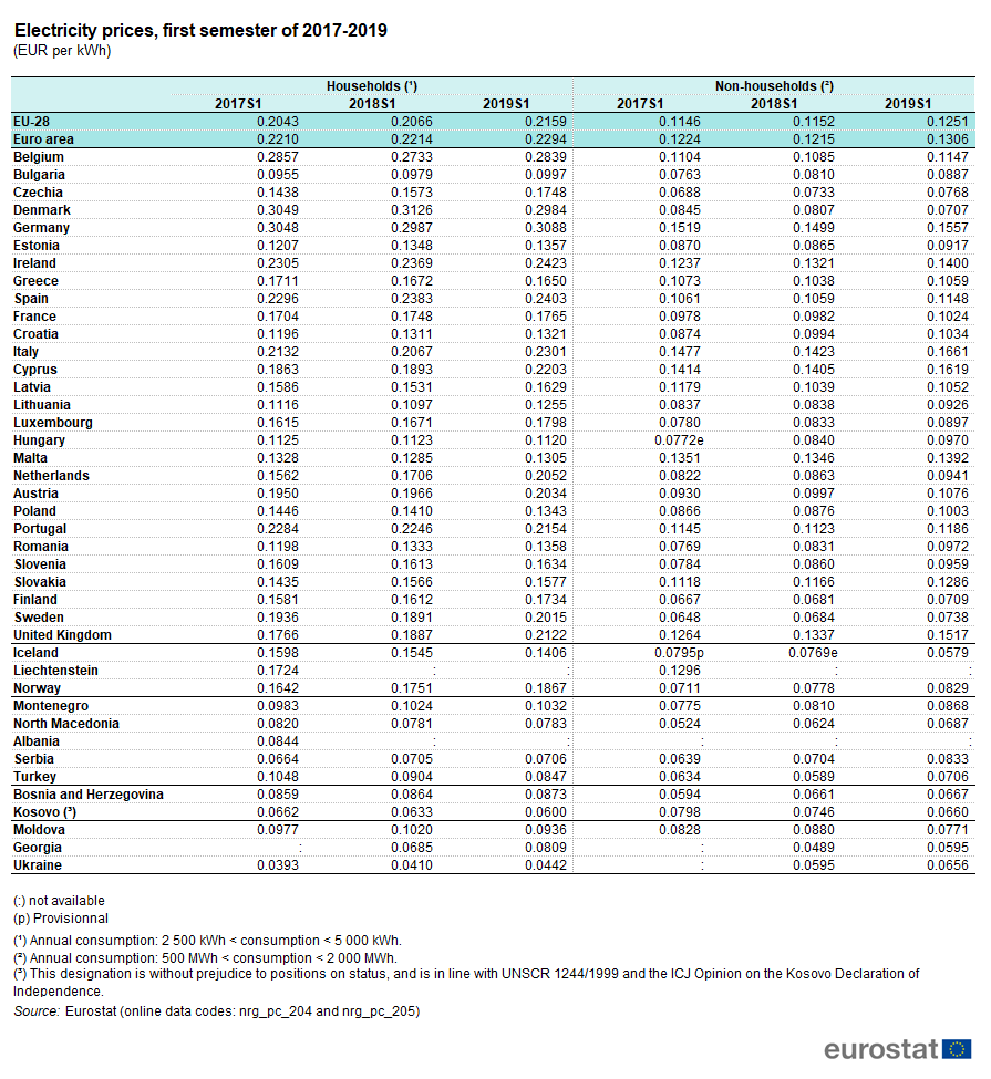
  Electricity grid: 0.24 * auto_calc (0.24 €/kWh is the average household electricity price of Spain for 2019S1. Obtained from Eurostat.)
  
  Gas plant: 0.0598 * auto_calc (0,0598 €/kWh for Germany and 0.072 €/kWh for Spain (2019 / 2020) - Values read in depending on location obtained from Eurostat’s statistic of gas prices)
2. feedin_tariff: currency/kWh,
  
  Electricity grid: (0.10 €/kWh is for Germany. We do not have data for Spain yet.)
  
  Gas plant: 0
3. inflow_direction: str,
  
  Electricity grid: Electricity
  
  Gas plant: Gas bus
4. label: str, Electricity grid feedin
5. optimizeCap: bool, True (for all of the components)
6. outflow_direction: str,
  
  Electricity grid: Electricity
  
  Gas plant: Heat bus
7. peak_demand_pricing: currency/kW, 0 (for all of the components)
8. peak_demand_pricing_period: times per year (1,2,3,4,6,12), 1 (for all of the components)
9. type_oemof: str, source (for all of the components)
10. energyVector: str, a. Electricity grid: Electricity b. Gas plant: Heat
11. emission factor: kgCO2eq/kWh a. Electricity grid: 0.338 b. Gas plant: 0.2 (Obtained from Quaschning 06/2015.)
energyStorage.csv:
1. inflow_direction: str, ESS Li-Ion
2. label: str, ESS Li-Ion
3. optimizeCap: bool, True
4. outflow_direction: str, ESS Li-Ion
5. type_oemof: str, storage
6. storage_filename: str, storage_01.csv
7. energyVector: str, Electricity
storage_01.csv:
1. age_installed: year, 0 (for all components)
2. development_costs: currency, 0 (for all components)
3. specific_costs: currency/unit
  
  storage capacity: 0.2 (Consult this reference https://www.energieheld.de/solaranlage/photovoltaik/kosten#vergleich for details.)
  
  input power and output power: 0
4. c_rate: factor of total capacity (kWh)
  
  storage capacity: NA (does not apply)
  
  input power and output power: 1 (this just means that the whole capacity of the battery would be used during charging and discharging cycles)
5. efficiency: factor
  
  storage capacity: 0
  
  input power and output power: 0.9 (Charging and discharging efficiency. The value has been sourced from this page.)
6. installedCap: unit, 0 (applies for all the parameters of the battery storage)
7. label: str, Same as the column headers (storage capacity, input power, output power)
8. lifetime: year, 10 (applies for all the parameters of the battery storage)
9. specific_costs_om: currency/unit/year, 0 (applies for all the parameters of the battery storage)
10. dispatch_price: currency/kWh
  1. storage capacity: NA (does not apply)
  2. input power and output power: 0
11. soc_initial: None or factor
  1. storage capacity: None
  2. input power and output power: NA
12. soc_max: factor
  1. storage capacity: 0.8 (Took the Fronius 4.5 battery which has a rated capacity 4.5 kW, but 3.6 kW is the usable capacity.So SoC max would be 80% or 0.8.)
  2. input power and output power: NA
13. soc_min: factor
  1. storage capacity: 0.1 (Figure from this research article.)
  2. input power and output power: NA
14. unit: str a. storage capacity: kWh
  1. input power and output power: kW
storage_02.csv:
1. age_installed: year, 0 (for all components of the stratified thermal storage)
2. development_costs: currency, 0 (for all components of the stratified thermal storage)
3. specific_costs: currency/unit
  
  storage capacity: 410, See Danish energy agency’s technology data of small-scale hot water tanks [dea_swt] on p.66 - However investment costs of stratified TES could be higher.
  
  input power and output power: 0
4. c_rate: factor of total capacity (kWh)
  
  storage capacity: NA (does not apply)
  
  input power and output power: 1 (this just means that the whole capacity of the stratified thermal storage would be used during charging and discharging cycles)
5. efficiency: factor
  
  storage capacity: 1, or “NA” if calculated
  
  input power and output power: 1
6. installedCap: unit 0, or “NA” if calculated
  
  storage capacity: 0, or “NA” if calculated
  
  input power and output power: 0
7. lifetime: year, 30 (applies for all the parameters of the stratified thermal energy storage)
8. specific_costs_om: currency/unit/year
  
  storage capacity: 16.67, [dea_swt] p.66 - however fix om costs of stratified TES could differ
  
  input power and output power: 0
9. dispatch_price: currency/kWh
  
  storage capacity: NA (does not apply)
  
  input power and output power: 0
10. soc_initial: None or factor
  1. storage capacity: None
  2. input power and output power: NA
11. soc_max: factor
  1. storage capacity: 0.925 (7.5% unused volume see European Commission study large-scale heating and cooling in EU [EUC_heat] p.168 - This applies for large scale TES but could be validated for a small scale storage too.)
  2. input power and output power: NA
12. soc_min: factor
  1. storage capacity: 0.075 (7.5% unused volume see [EUC_heat] p.168 - This applies for large scale TES but could be validated for a small scale storage too.)
  2. input power and output power: NA
13. unit: str
  1. storage capacity: kWh
  2. input power and output power: kW
14. fixed_thermal_losses_relative: factor
  1. storage capacity: “{‘file_name’: ‘None’, ‘header’: ‘no_unit’, ‘unit’: ‘’}”, is calculated in pvcompare
  2. input power and output power: NA (does not apply)
15. fixed_thermal_losses_absolute: kWh
  1. storage capacity: “{‘file_name’: ‘None’, ‘header’: ‘no_unit’, ‘unit’: ‘’}”, is calculated in pvcompare
  2. input power and output power: NA (does not apply)

2. pvcompare-specific parameters¶

In order to run pvcompare, a number of input parameters are needed; many of which are stored in csv files with default values in pvcompare/pvcompare/inputs/. The following list will give a brief introduction into the description of the csv files and the source of the given default parameters.

pv_setup.csv:
The pv_setup.csv defines the number of facades that are covered with pv-modules.
1. surface_type: str, optional values are “flat_roof”, “gable_roof”, “south_facade”, “east_facade” and “west_facade”
2. surface_azimuth: integer, between -180 and 180, where 180 is facing south, 90 is facing east and -90 is facing west
3. surface_tilt: integer, between 0 and 90, where 90 represents a vertical module and 0 a horizontal.
4. technology: str, optional values are “si” for a silicone module, “cpv” for concentrator photovoltaics and “psi” for a perovskite silicone module
building_parameters:
Parameters that describe the characteristics of the building that should be considered in the simulation. The default values are taken from [1].
1. number of storeys: int
2. population per storey: int, number of habitants per storey
3. total storey area: int, total area of one storey, equal to the flat roof area in m²
4. length south facade: int, length of the south facade in m
5. length eastwest facade:int, length of the east/west facade in m
6. hight storey: int, hight of each storey in m
7. room temperature: int, average room temperature inside the building, default: 20 °C
8. heating limit temperature: int, temperature limit for space heating in °C, default: 15 °C
9. include warm water: bool, condition about whether warm water is considered or not, default: False
10. filename_total_consumption: str, name of the csv file that contains the total electricity and heat consumption for EU countries in different years from [2] *
11. filename_total_SH: str, name of the csv file that contains the total space heating for EU countries in different years [2] *
12. filename_total_WH: str, name of the csv file that contains the total water heating for EU countries in different years [2] *
13. filename_elect_SH: str, name of the csv file that contains the electrical space heatig for EU countries in different years [2] *
14. filename_elect_WH: str, name of the csv file that contains the electrical water heating for EU countries in different years [2] *
15. filename_residential_electricity_demand: str, name of the csv file that contains the total residential electricity demand for EU countries in different years [2] *
16. filename_country_population: str, name of the csv file that contains population for EU countries in different years [2] *
heat_pumps_and_chillers:
Parameters that describe characteristics of the heat pumps and chillers in the simulated energy system. Values below assumed for each heat pump technology from research and comparison of three models, each of a different manufacturer. For each technology the quality grade has been calculated from the mean quality grade of the three models. Maximal and minimal operation ranges had been considered in order to make a reasonable assumption regarding temp_high and temp_low .
1. mode: str, options: ‘heat_pump’ or ‘chiller’
2. technology: str, options: ‘air-air’, ‘air-water’ or ‘brine-water’ (These three technologies can be processed so far. Default: If missing or different the plant will be modeled as air source) 2. quality_grade: float, scale-down factor to determine the COP of a real machine (Can be calculated from COP provided by manufacturer under nominal conditions and nominal temperatures. Required equations can be found in the oemof.thermal documentation of compression heat pump and chiller.)
air-to-air heat pump: default: 0.1852, Average quality grade of the following heat pump models: RAC-50WXE Hitachi, Ltd., MSZ-GL50 Mitsubishi Electric Corporation and KIT-E18-PKEA of Panasonic Corporation

air-to-water heat pump: default: 0.4030, Average quality grade of the following heat pump models: WPLS6.2 of Bosch Thermotechnik GmbH – Buderus, WPL 17 ICS classic of STIEBEL ELTRON GmbH & Co. KG and 221.A10 of Viessmann Climate Solutions SE

brine-to-water heat pump: default: 0.53, Average quality grade of the following heat pump models: WPS 6K-1 of Bosch Thermotechnik GmbH – Buderus, WPF 05 of STIEBEL ELTRON GmbH & Co. KG and 5008.5Ai of WATERKOTTE GmbH

air-to-air chiller: 0.3 (Obtained from monitored data of the GRECO project)
1. temp_high: float, temperature in °C of the sink (external outlet temperature at the condenser),
  
  air-to-air heat pump: 26 (Maximal operation temperature in data sheet of RAC-50WXE Hitachi)
  
  air-to-water heat pump: 60 (Maximal operation temperature in data sheet of 221.A10 of Viessmann Climate Solutions SE)
  
  brine-to-water heat pump: 65 (Maximal operation temperature in data sheet of WPF 05 of STIEBEL ELTRON GmbH & Co. KG)
  
  air-to-air chiller: Passed empty or with NaN in order to model from ambient temperature
2. temp_low: float, temperature in °C of the source (external outlet temperature at the evaporator),
  
  air source heat pump: Passed empty or with NaN in order to model from ambient temperature
  
  air-to-water heat pump: Passed empty or with NaN in order to model from ambient temperature
  
  brine-to-water heat pump: Passed empty or with NaN in order to model from mean yearly ambient temperature as simplifying assumption of the ground temperature from depths of approximately 15 meters (see brandl_energy_2006)
  
  air-to-air chiller: 15 (The low temperature has been set for now to 15° C, a temperature lower the comfort temperature of 20–22 °C. The chiller has not been implemented in the model yet. However, should it been done so in the future, these temperatures must be researched and adjusted.)
3. factor_icing: float or None, COP reduction caused by icing, only for mode ‘heat_pump’, default: None
4. temp_threshold_icing: float or None, Temperature below which icing occurs, only for mode ‘heat_pump’, default: None
list_of_workalendar:

list of countries for which a python.workalendar [3] exists with the column name “country”.

[1] Hachem, 2014: Energy performance enhancement in multistory residential buildings. DOI: 10.1016/j.apenergy.2013.11.018

[2] EUROSTAT: https://ec.europa.eu/energy/en/eu-buildings-database#how-to-use

[3] Workalendar https://pypi.org/project/workalendar/

* the described csv files are to be added to the input folder accordingly.

Simulation outputs¶

The following image shows a schematic figure of how the output structure of pvcompare is composed.

Composition of the output structure within pvcompare.

For each scenario, a specific output folder with the name scenario_name is created. All outputs are saved into this scenario_folder. When running apply_mvs() all outputs created by mvs are saved into the folder mvs_outputs. When running loop_mvs() a loop output directory with the additional information of the variable name that is looped over, is created. Within this loop_output_directory all time series and all scalars are copied into specific folders and named with their specific looping step. Additionally all mvs_outputs are saved into a folder with the name `mvs_outputs_loop_variable_name_step’, so that the specific steps can be analyzed easily in separate. For each scenario multiple loops can be applied.

The following image shows an example output directory with specific names of the folders. In this example the function apply_mvs() was run. Further one loop for specific costs over two values (500, 600) was executed.

Example output structure of pvcompare with one loop over specific costs.

Definition of KPIs¶

KPIs, which were calculated from the outputs of the simulation, are stored in Scalars. The main ones used to interpret the results of simulated scenarios are presented in this section.

Self-consumption also onsite energy fraction is defined as the fraction of all locally generated energy that is consumed by the system itself to the system’s total local generation:

$Self\_Consumption &=\frac{\sum_{i} {E_{generation} (i)} - E_{gridfeedin}(i) - E_{excess}(i)}{\sum_{i} {E_{generation} (i)} } &Self Consumption \epsilon \text{[0,1]}$

The degree of autonomy is used to describe all locally generated energy that is consumed by the system over the system’s total demand:

$Degree\_Of\_Autonomy &=\frac{\sum_{i} {E_{generation} (i)} - E_{gridfeedin}(i) - E_{excess}(i)}{\sum_i {E_{demand} (i)}} &Degree of Autonomy \epsilon \text{[0,1]}$

With the degree of net zero energy , the margin between grid feed-in and grid consumption is compared to the overall demand:

$Degree\_Of\_Net\_Zero\_Energy = 1 + \frac{\sum_{i} E_{gridfeedin}(i) - E_{consumption,provider}(i)}{\sum_{i} E_{demand} (i)}$

Please see the section Outputs of the MVS simulation / Technical data of MVS’s documentation to learn more about the degree of net zero energy.

Scope and limitations¶

The pvcompare model was developed during the H2020 project GRECO with the purpose of analysing the integration of three innovative PV techologies, that are developed within the project, into energy systems in comparsion to the state-of-the-art technology. These three technologies are

contentrator-PV (CPV),
a multi-junction of perovskite and silicon (PSI) and
PV powered heat pumps and chillers.

Therefore, the model focuses on Photovoltaiks, while also including sector-coupling through heat pumps and chillers. However, a shift of focus is possible and can easily integrated. Feel free to contribute and check out our Contributing Guidelines.

More information on the scope and limitations will follow.

GRECO Results¶

Here we will publish selected scenarios that we simulated for the H2020 Project GRECO and their results, which will also serve as examples.

Results of PV modeling¶

In PV Modeling the models used to generate feed-in time series for SI, CPV and PSI technologies are presented. This section will show some results of the calculated time series and discuss model assumptions.

The generated hourly time series over one year are normalized by the peak power of each module. Figure PV time series shows an exemplary time series for all three technologies in year 2014 in Madrid.

Normalized time series for Madrid, Spain in 2014.

Figure Daily Profiles shows the daily profiles of all three technologies. It demonstrates how the CPV technology has a more narrow profile, because it highly depends on the DNI. Further, the profile of PSI exceeds the SI profile in the middle of the day. It can be seen nicely how the profiles are shifted on the east and west facade due to the solar position. The profiles are normalized with their maximum value in order to compare them conveniently.

Daily profiles of all three technologies, Spain 2014.

Daily profiles (normalized with maximum value) of SI, PSI and CPV for south, east and west orientation, Spain in 2014.

Energy yield¶

The size and efficiency of the three modules used age given in table1.

Figure energy yield shows the yearly energy yield per kWp on the left-hand side and the yearly energy yield per m² on the right-hand side. The plot shows that the production per kWp is the highest for SI. This is due to a high performance ratio of SI. The lower performance ratio of Hybrid CPV results in a lower production per kWp. Nevertheless, when looking at the production per m², the Hybrid CPV technology as well as the PSI technology perform better than SI, due to it’s higher efficiency (Wp per m²). Overall, as expected, the yield in Berlin is lower than in Madrid but also the margin between the technologies decreases in Berlin. This outcome is due to a lower direct normal irradiance (DNI) in Berlin which causes a decrease in the yield of the Hybrid CPV technology.

Energy yield per kWp (left) and per m² (right) for Berlin and Madrid in 2014.

Hybrid CPV¶

Figure CPV - Flatplate profile shows the daily production of a single CPV and Flatplate panel for Spain in 2014. The figure shows how the flatplate produces only in the morning and the evening, because it is restricted to a solar angle > 60°. The CPV component has a more narrow peak in the middle of the day, when the DNI has its maximum.

Electricity production of Flatplate and CPV component and irradiance (DHI, DHI) in Madrid, Spain in 2014.

Figure Hybrid CPV illustrates the energy yield for the different components of the Hybrid CPV technology. The Flatplate component collects diffuse horizontal irradiance (DHI) while the CPV components only collects direct normal irradiance (DNI). The Hybrid module adds up both power outputs of the Flatplate and the CPV part. For more information about the modeling of Hybrid CPV see PV Modeling.

Yearly energy yield of the Hybrid CPV and its components per m² for Berlin and Madrid in 2014.

Code documentation¶

Main¶

Main functions of pvcompare that can be used to start a full simulation.

`main.main`
`main.apply_mvs`

Area potential¶

Function for calculating the area potential of the rooftop and facades for a given population.

area_potential.calculate_area_potential

Demand¶

Functions for calculating the electrical demand profiles and heat demand profiles.

`demand.calculate_load_profiles`
`demand.calculate_power_demand`
`demand.calculate_heat_demand`
`demand.shift_working_hours`
`demand.get_workalendar_class`

Feed-in time series of photovoltaic installations¶

Functions for calculating the feed-in time series of different PV technologies.

`pv_feedin.create_pv_components`
`pv_feedin.create_si_time_series`
`pv_feedin.create_cpv_time_series`
`pv_feedin.nominal_values_pv`
`pv_feedin.set_up_system`
`pv_feedin.get_optimal_pv_angle`

CPV time series¶

Function for calculating the feed-in time series for the CPV technology.

cpv.apply_cpvlib_StaticHybridSystem.create_cpv_time_series

PSI time series¶

Function for calculating the feed-in time series for the perovskite silicone technology.

`perosi.perosi.create_pero_si_timeseries`
`perosi.perosi.create_timeseries`
`perosi.perosi.calculate_smarts_parameters`
`perosi.pvlib_smarts.SMARTSSpectra`
`perosi.pvlib_smarts._smartsAll`

Reading and Writing input csv’s¶

Functions that match manual inputs and calculated results with mvs_inputs/csv_elements/

`check_inputs.check_for_valid_country_year`
`check_inputs.add_project_data`
`check_inputs.add_electricity_price`
`check_inputs.check_mvs_energy_production_file`
`check_inputs.add_parameters_to_energy_production_file`
`check_inputs.add_evaluated_period_to_simulation_settings`

Loading ERA5 weather data¶

Functions that request the weather data of one year and one location from the ERA5 weather data set

`era5.load_era5_weatherdata`
`era5.get_era5_data_from_datespan_and_position`
`era5.format_pvcompare`
`era5.weather_df_from_era5`

Output functions¶

`outputs.loop_mvs`
`outputs.plot_all_flows`
`outputs.plot_kpi_loop`

Troubleshooting¶

Problems during the installation were observed on a python 3.7 environment with these two packages:

psycopg2
graphiz

on the following system:

Operating System:
Kernel: Linux 5.4.0-66-generic
Architecture: x86-64

Running a simulation may error out. In this case the two packages must be installed in an alternative way, for instance using conda:

conda install -c anaconda psycopg2
conda install -c anaconda graphviz